

The COVID-19 pandemic has affected the lives and habits of billions of people around the world. One of the newly observed trends is the apparent increase in interest in financial markets, as illustrated in Figure 1.
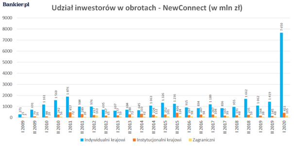
It is impossible not to notice the fivefold increase in turnover generated by individual investors or, to put it another way, “ordinary Kowalskis”. A similar trend is also observed on cryptocurrency exchanges. There are many reasons for this. One of them may be the desire to protect capital against a potential economic crisis or high inflation.
Leaving aside the reasons, it is worth asking a question – what could be the consequences? One of them is the emergence of a number of inexperienced investors, whose lack of familiarity with the market realities may pose a serious threat in the face of not always legal practices of some market participants.
Pump & Dump (Mechanism Description)
Pump & Dump is the name of the process of manipulating the valuation of an asset in the market. It consists of artificially inducing a price increase by creating the illusion of sudden interest in shares of a given company. When the price reaches a high enough level, the person organizing the shares sells the previously acquired claims at an inflated price.
Let’s break down the mechanism into stages:
- Generating increased traffic in the company by buying back shares.
- After two or three days of continuous growth caused by the buyback, the company attracts the attention of other market participants who, wanting to take advantage of the price increase, issue purchase offers.
- When a sufficient number of investors become interested in the company, the organizer buys many shares, “clearing” the queue. This results in a rapid increase in the stock price. Other players seeing the dynamics, also want to become owners of the company’s shares, raising the price even higher. The bubble begins to live its own life – it propels itself.
- After reaching an appropriate price ceiling, the organizer gradually get rid of his shares, selling them at an inflated price.
- The next few days bring a correction and the price returns to the level from before the action.
For the operation to be possible, the company’s victim (the attack) must meet several criteria.
First of all, capitalization must be sufficiently low, which reduces the amount of capital required to act. The second criterion is the liquidity of the company. Here, ideally, it should be low and still exist. This makes it possible to generate movement in phase one while our trades are dominant in the company.
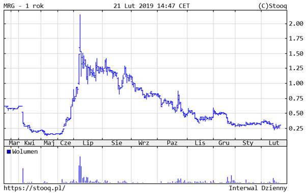
FIg 2: Example of Pump&Dump suspect quotes
Machine learning
The increase in computing power of computers over the past few years and the progressive digitization of data have created conditions conducive to the development of advanced forms of data analysis, in particular artificial intelligence algorithms have benefited. In a nutshell, to reap the benefits of so-called models, we need to train them beforehand, that is “show” historical data related to the problem under study. This can be accomplished in several ways. The two most popular are so-called supervised learning and unsupervised learning. With the former you are required to specify a class for each observation – what is visible in the image, what the text is about or whether the transaction is fraudulent.
In unsupervised techniques we are limited to just the data itself without specifying the class of each observation. As is usually the case each approach has its pros and cons. Often, creating the data description necessary to apply supervised techniques is a labor- and time-intensive activity, often involving many people with specific skills. Naturally this increases the cost of the project and the time to complete it.
From this perspective unsupervised learning seems better. However, this is not the whole truth. Unsupervised algorithms usually work based on similarity. The group data into clusters that combine the most similar observations or identify outliers.
Unfortunately, the Data Scientist has limited control over this process, which means that the model may pay attention to different aspects of the data than the author’s intentions would suggest. This usually means less accurate predictions, which translates into poorer results than to supervised methods. On the other hand, the lack of a requirement to label each observation reduces data preparation time.
It may also happen that leaving the interpretation of the data to the model will lead to the discovery of correlations previously overlooked or erroneously ignored by the Data Scientist. Nevertheless, in practice, solutions based on supervised learning are preferable because of the greater control over the learning process, the possibility of adapting the classes of observations to the analyzed problem and better results.
Implementation
Let us consider the possibility of automatic detection of Pump & Dump practices described earlier. Undoubtedly, the mechanism’s characteristics are strong increases in price and volume. At the same time, we do not have an official database of identified manipulation cases.
It would take weeks of work for a person skilled in detecting stock market irregularities to flag all available data manually. Such an undertaking is beyond the scope planned for the current article. In line with the earlier description of machine learning techniques, I will focus on unsupervised type algorithms.
These carry the risk of unintentionally indicating correct quotes as instances of manipulation. This is due to the high similarity of Pump & Dump to the situation that may occur, for example, after the publication of unexpectedly good financial results of a company. Possible nuances that distinguish these two cases may not be considered by the model which the Data Scientist has limited influence on. With all the knowledge presented so far, let’s try to build an artificial intelligence model whose task will be to detect unusual events.
GAN
Generative Adversarial Networks, or GAN for short, is a way of training machine learning models where two networks compete against each other. The task of one of them (generator) is to generate observations, while the other network (discriminator) tries to distinguish actual observations from generated ones. As a training set (real observations for the discriminator), we use historical quotations of companies from the NewConnect exchange, divided into 5 to 90 days sequences.
Companies listed on NewConnect seem to be a better testing ground than those from the more widely known main market of the Warsaw Stock Exchange. This is due primarily to their more susceptibility to Pump & Dump attacks. Compared to their counterparts from the WSE, they are characterized by lower capitalization, liquidity and popularity.
In turn, the length of the sequence results from the observation of historical quotations. It is impossible to unequivocally state the manipulation operation begins and when it ends. Nevertheless, 5 consecutive quotes seem to be the minimum value. Longer/More extended periods are intended to supplement the data with a broader context.
| Sequence length | Training set size | Test set size |
|---|---|---|
| 5 | 499 932 | 11 985 |
| 30 | 12 026 | 11 785 |
The idea behind the proposed solution is quite simple. The stock price series produced by the generator become similar to real to fool the discriminator. Since non-standard rate/volume changes are relatively rare, both networks adapt to the standard series. This means that a trained discriminator should flag the Pump & Dump case as “fake”.
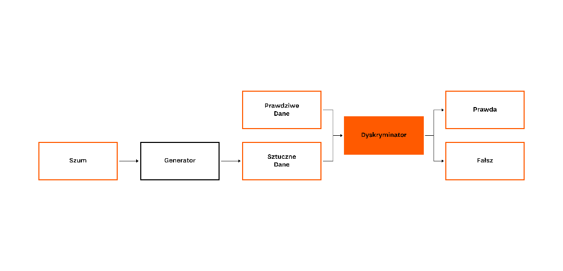
Fig 3: Functional diagram of GAN type architecture
The process of optimizing the solution was done iteratively, starting with training on a severely limited amount of data and a smaller network, which was gradually increased when the overfitting point was reached. I prepared a small test set for evaluation purposes where I manually flagged suspicious cases captured on the NewConnect exchange.
The first approach – Fully Connected layers
building blocks of a discriminator and generator within the GAN architecture. Their ability to “remember” observations gave very good results in the initial stage (for a limited number of observations). Unfortunately, they performed poorly when generalizing to larger amounts of data.
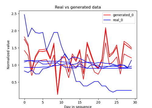
Fig 4: Example sequence generation (closing quotation data). The resulting quotes exhibit strong similarity, which contrasts strongly with the diversity of the true runs.
Second approach – LSTM
Due to the nature of the analyzed data (time series), it seems natural to use recursive layers, more specifically LSTM (Long Short Term Memory). Their main advantage is that they take into account the entire series of points, not just a single observation. The mentioned functionality is realized by a system of gates, which combine the incoming data with the information obtained from the previous points of the sequence.
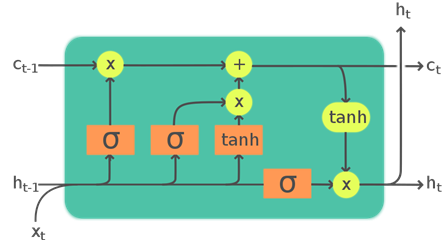
Fig 5: Schematic of how an LSTM cell works. Source: https://upload.wikimedia.org/wikipedia/commons/9/93/LSTM_Cell.svg
Unfortunately, as in the previous case, the results are not satisfactory. I tested both approaches with a Fully Connected generator and LSTM discriminator and one where both networks were based on LSTM.
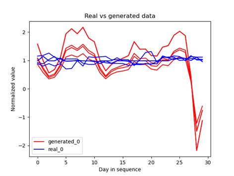
Fig 6: Generated sequences for closing prices and volume
Third Approach – Convolution
Convolutional (convolutional) networks are commonly used image processing, NLP or graph networks. Due to the topic of this paper, we will use them to interpret time series. For the case study I used the so-called “Causal Convolution”.
The standard convolution operation, applied to a one-dimensional time series, considers both the points located “before” and “after” the point for which the convolution is calculated, in this particular case called one-dimensional. Let’s analyze this using the example in the figure below.
Our series is a sequence of numbers one per day (green). We apply a convolution with a kernel dimension equal to 3, symbolically represented by the gray color and arrows. This means that when calculating a new series, the value for day 11.07.2021 is calculated using the data from days 10.07.2021, 11.07.2021, and 12.07.2021.
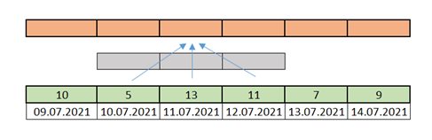
Fig 7: An example of using classical convolution for the case of a time series
As we can see, classical convolution combined with ordered data raises the problem of “looking” into the future. Causal Convolution limits the input data only to those “historical”, thus preserving causality. This is realized through an asymmetric weave kernel that only considers past data.
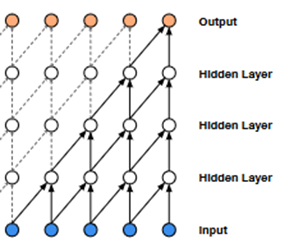
Fig 8: WaveNet: A Generative Model for Raw Audio
The results obtained in this way looked relatively most attractive.
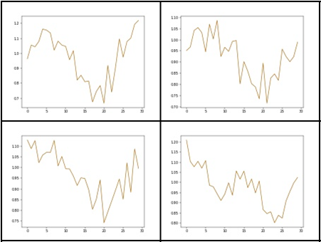
Fig 9: Results obtained using one-dimensional convolution
Results
Obtaining a network that generates realistic-looking stock quotes is not a simple issue. Although it is a kind of by-product of discriminator training, it can be treated as a good indicator of the quality of a GAN-type network. Unfortunately, the generated stock price series did not resemble real quotations in most of the conducted training. Additionally, the quality of the obtained results was affected by the so-called “mode collapse” phenomenon, which causes a reduction in the diversity of the data coming from the generator.
The results obtained on the test set were characterized by a significant scatter. Depending on the training time, the same discriminator model could indicate all observations from the test set as false, true or doing it in a completely unexpected way. Therefore, it is hard to talk about any particular metric value. Alternatively, the high classification score obtained (e.g., AUC above 0.8) could be due to the discriminator adjusting randomly to a relatively small test set.
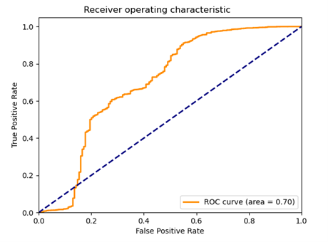
Fig 10: Example ROC plot for the models studied
Classic methods
Let’s verify the ability to detect unusual events using more established techniques – classical machine learning and rule sets. To do this I will change the data format slightly. A single observation in the set will be a quotation from a given day and features describing the change in the value of a given stock. Of course, this will affect the size of the datasets.
| Training set size | Test set size |
|---|---|
| 468 663 | 10 783 |
Modeling
Let us first take the Isolation Forest algorithm. Its goal is to identify unusual observations in a set. In a nutshell, the algorithm splits based on a selected variable’s value. The feature’s choice and the value against which the division takes place are chosen randomly. Outliers need significantly less number of splits to be isolated. Let us verify the effectiveness of Isolation Forrest on a group of companies that we suspect are victims of the Pump & Dump attack.
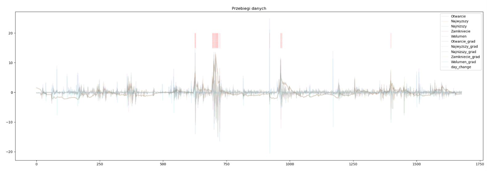
Fig 11: Quotations of one of the companies with the points indicated by the model
In the chart above (Figure 11), we see the quotes and their derivatives for one of the companies. The operations to which the original data have been subjected are mainly the standardization of the range and the determination of daily differences (gradients). Cases identified as outliers are marked with red lines at the chart’s top. The model seems to have done quite well – detecting anomalies in the observed data. A similar observation emerges after examining the second graph, i.e. Figure 12.
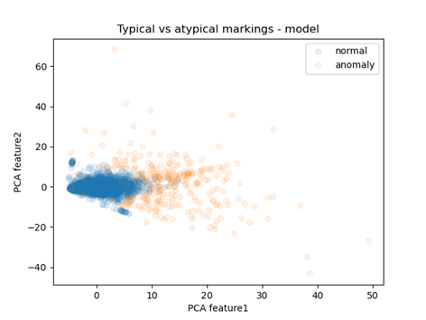
Fig 12: Distribution of points in reduced space
I used the PCA algorithm to produce it, which reduced the number of dimensions to two (previously non-existent), allowing for a readable visualization. Each point represents one observation. The colors distinguish whether it was considered normal or abnormal. There is a clear concentration of blue points, while those representing abnormal observations are much further from the center. This confirms the effectiveness of the model in identifying abnormal observations.
Finally, we plot the confusion matrix and ROC for the test set:
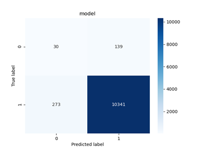
Fig 13: Confusion matrix for the Isolation Forest model
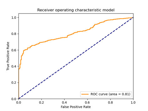
Fig 14: ROC diagram for the analyzed model
Rule set
The methods described so far do not exhaust all available solutions. To increase the completeness of the analysis of the problem, it is worth confronting the results with the approach based on a set of rules. It is the simplest conceptually, which does not necessarily mean worse results.
As a determinant of “normality” I used the sum of distances of a given observation from the mean expressed in units of standard distance. For example, for the case of observations where the value of the first characteristic is 5, the mean is 3, and the standard deviation is 2, the result is:
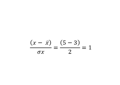
The operation is repeated for the remaining features and the absolute values are summed. The two graphs below show the distribution of the obtained results appropriate for sums and single columns.
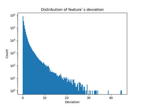
Fig 15: The distribution of the distance of the value of a trait from its mean expressed in units of standard deviation. Logarithmic scale
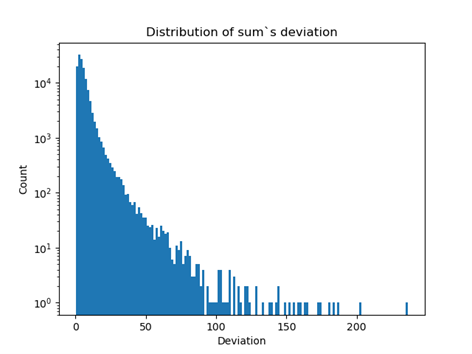
Fig 16: The distribution of the sum of distances of a feature from its mean expressed in units of standard deviation. Logarithmic scale
As expected, the distribution is strongly clustered around low values. As a criterion for belonging to the anomalous group, I observed a value exceeding the 99th centile for the sum of distances or any feature describing a single quotation. Below, we see analogous visualizations for the Isolation Forest model approach. It seems that the results obtained using rules are slightly worse.
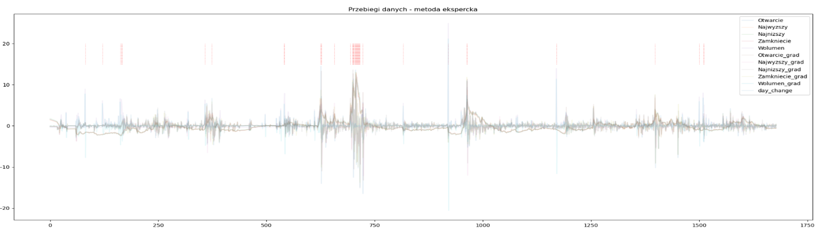
Fig 17: Quotations of one of the companies with the points indicated by the rule set
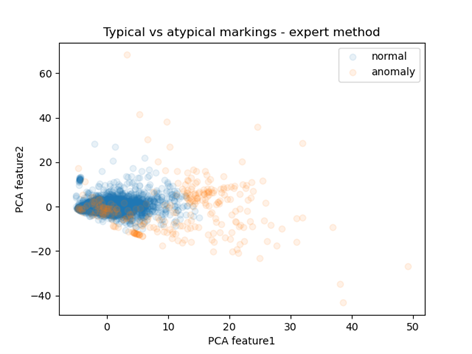
Fig 18: Prediction distribution in space reduced using PCA
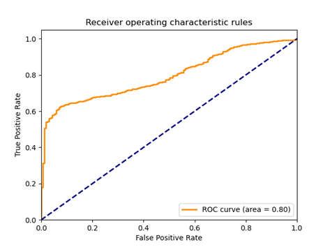
Fig 19: AUC plot for the test set

Fig 20: Classification results on the test set obtained for the rule set model
Conclusions
The work done in the paper can be divided into two areas – generation of quotations and detection of unusual cases. The former is not a simple task. Training models based on GANs architecture involve many problems, such as selecting properly balancing discriminator and generator, optimal training parameters, etc. Nevertheless, the solution using Causal Convolution networks can serve as a starting point for further research in this direction. The results obtained in this way looked quite realistic.
In detecting Pump & Dump practices, the standard anomaly detection methods – Isolation Forest and rule set – performed better. On a pre-prepared test set they achieved results that can attest to the usefulness of the models. At the same time, it should be noted that there is no official data on the detection of the described practices and the scale of the procedure and thus, a well-defined set. Not every significant jump of quotations or volume of transactions must mean illegal practices, introducing another degree of difficulty to the overall solution.
In conclusion, the described and the application of unsupervised machine learning techniques have managed to track down probable cases of stock market manipulation. As expected, the results obtained are subject to inaccuracies due to the nature of unsupervised learning.